


Neural networks are at the heart of modern artificial intelligence. They allow machines to learn from data, and they’re everywhere: voice assistants, machine translation, image recognition, recommendations, and text generation.
To understand how these systems work — and their limits — a short historical detour helps set the foundations.
A brief history of artificial intelligence
AI was officially born in 1956 at the Dartmouth conference: researchers imagined that a machine could one day simulate human intelligence.
In the 1960s, the perceptron appeared, an ancestor of neural networks. The idea was simple: take numerical inputs and produce a decision. But at the time, there wasn’t enough data or computing power. Progress slowed.
This led to the first AI winter in the 1970s: funding dropped and research stalled. A revival came in the 1980s thanks to a key concept: backpropagation. But momentum faded again at the end of the decade.
Everything changed in the 2010s because three factors aligned:
- We have massive amounts of data
- GPUs can compute very quickly
- Networks are getting faster and more powerful
From 2020 onward, generative AI became accessible to the general public. Neural networks entered a new phase: widespread adoption and real-world use cases. This is the rise of OpenAI, Mistral, Grok…
What is a neural network?
Let’s go back to basics to understand what we’re doing today! A neural network is a set of small computing units called artificial neurons, organized into layers and connected to each other.
Each neuron performs a very simple calculation. But when you combine thousands (or millions…) of them, complex behavior emerges.
The idea is simple: a neuron transforms input values into an output value.
A neuron: a mini-function
A neuron receives one or more inputs:
x1, x2, x3… (pixels, measurements, words turned into numbers)
Each input has a weight:
w1, w2, w3…
The weight indicates the importance of the input.
The neuron computes a weighted sum:
x1w1 + x2w2 + x3w3 + …
Then it adds a bias b, which shifts its behavior:
z = (x1w1 + x2w2 + …) + b
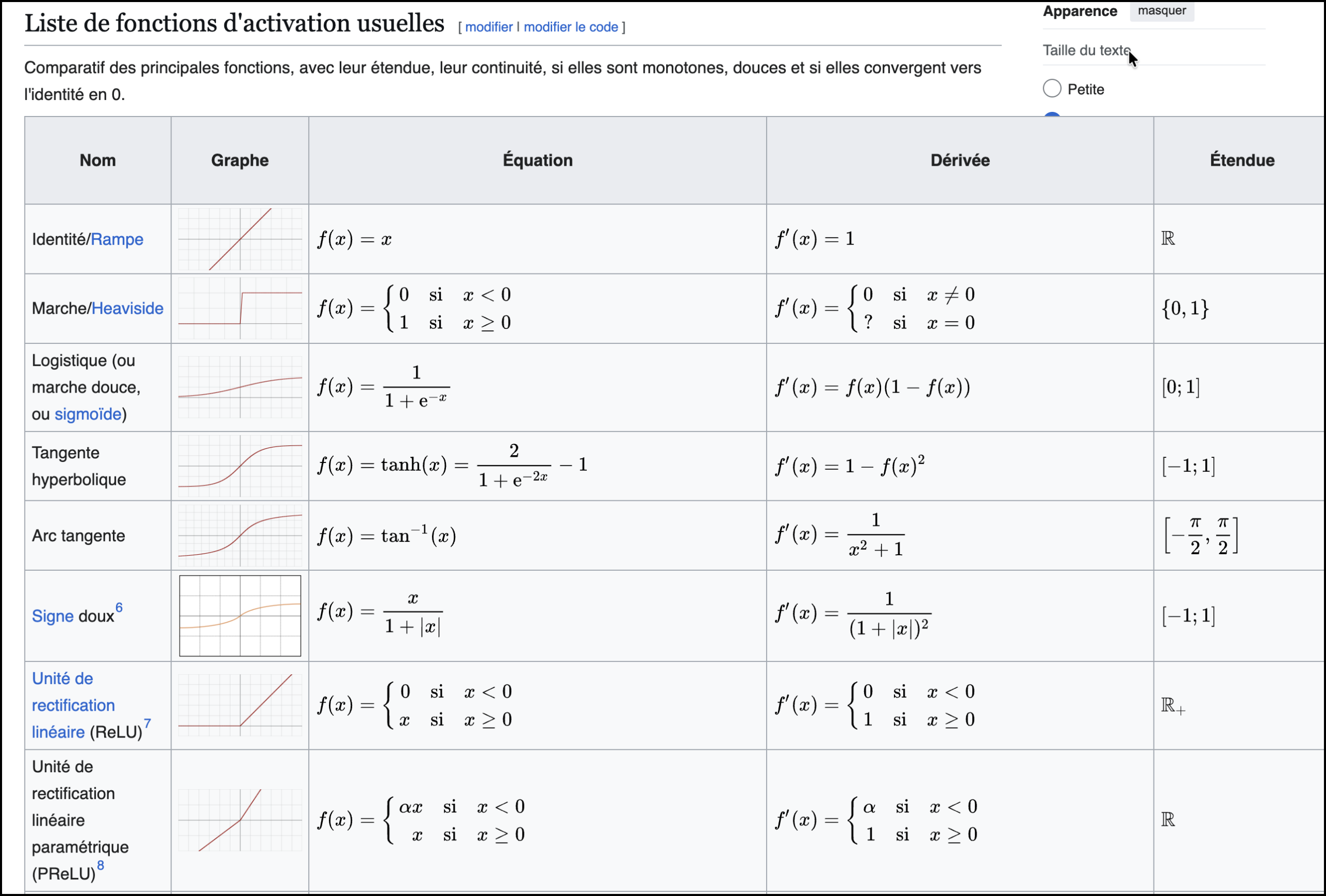
Finally, it applies an activation function:
y = f(z)
This activation plays a crucial role: it allows the network to model complex relationships, not just additions. It determines whether the neuron is activated and how it contributes to the final result.
Excerpt from Wikipedia
In short:
✅ Inputs → weighting → sum → activation → output
Network = neurons in a chain
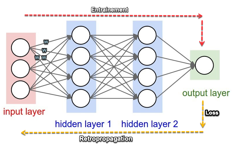
A neural network is a stack of layers:
- input layer: receives the data
- hidden layers: transform the information
- output layer: produces the result
In computer vision for example, the network can gradually learn:
- edges and contrasts
- patterns (shapes, textures)
- objects (“cat”, “car”, etc.)
Why are weights essential?
Weights are what the model learns.
They literally make up its “memory”.
When a network learns, it doesn’t add explicit rules.
It adjusts its weights to produce better outputs and statistically get closer to the expected result.
Simple diagram (web version)
x1 ──(w1)─┐
x2 ──(w2)─┼──▶ sum + bias ─▶ activation f(z) ─▶ y
x3 ──(w3)─┘

Do you know the game Plinko?
A neural network is a bit like a game of Plinko. You know that game where a ball falls through a board full of pegs.
With each bounce, it deviates slightly… and eventually lands in an output slot.
Imagine an input data point entering a neural network. It goes through the layers, gets modified by neurons, and reaches the output with a targeted value. The network’s job is to adapt so that the ball always falls into the right slot — the one that wins!
Indeed:
- each local interaction is simple
- but the sum of bounces produces a global result
A neural network works similarly:
- each neuron performs a small local calculation
- no neuron “understands” the final result
- but together they produce a coherent output
And most importantly: changing the Plinko board changes the trajectory.
In a network, changing the weights and activation function changes the model’s behavior.
✅ Key takeaways — Neural network
- A neuron = a function: weighted sum + activation
- Weights determine the importance of inputs
- Learning = adjusting the weights
- Many simple neurons → complex behavior
How does a neural network learn?
To learn, the network makes predictions on a dataset, then compares its results to the correct answer.
The difference is measured by a loss function.
Loss: measuring the error
👉 Loss is a number that measures “how wrong the network is”. I’ll skip the loss computation algorithms, which would require a whole article by themselves.
- high loss → bad prediction
- low loss → good prediction
The goal of training is simple: ✅ reduce the loss
How to adjust weights efficiently?
Once the loss is computed, the network must know how to modify the weights to improve.
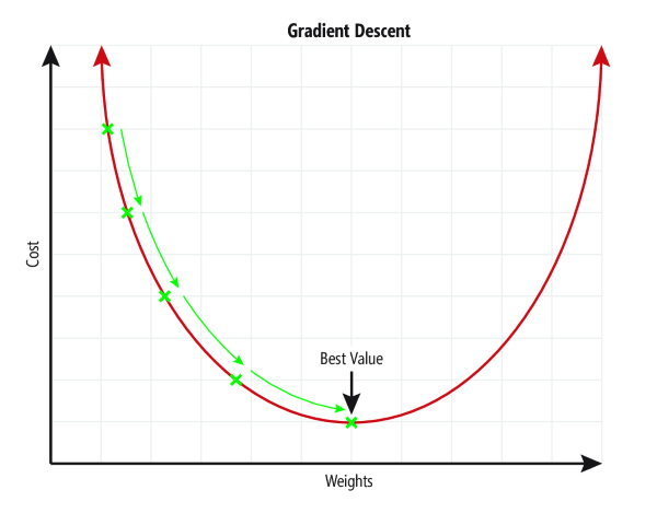
That’s the role of gradient descent. Again, this algorithm aims to find the best weight value for each neuron.
The detailed explanation is quite complex but available online, on Wikipedia for example:
https://fr.wikipedia.org/wiki/R%C3%A9tropropagation_du_gradient
Note that this algorithm plays a crucial role due to the step size needed to reach the best value (see the curve).
Indeed:
- too small → stable, but slow
- too large → unstable, the model “jumps” around the solution
Once these concepts are understood, we begin training the model on the dataset. We make it process the data many times so it can adjust the network and reach what it considers the best solution. These multiple passes over the dataset are what we call the number of training epochs.
An epoch
An epoch = one full pass over all training data.
Example:
- 10,000 images
- 20 epochs
- the model has seen those images 20 times
✅ More epochs = more chances to learn
⚠️ Too many epochs = risk of overfitting
In practice, we don’t process all the data at once.
We split it into mini-batches:
- after each mini-batch, weights are adjusted
- one epoch corresponds to a full pass through all mini-batches
Train / Validation / Test
It’s time to check the quality of our work. To verify whether the model is truly good, we split the data into three sets:
- Train: the model learns — we provide questions and answers
- Validation: we check during training — we still provide questions and answers
- Test: final evaluation — on never-seen data — we only provide the questions and compare to expected answers
train = exercises
validation = practice exams
test = final exam
This step is essential to detect overfitting or over-specialization.
I once read an anecdote about training a model whose job was to detect images of huskies. During training the results were excellent. During tests, still excellent. In production it became really bad.
After investigation, the reason was simple: the network hadn’t learned to recognize a husky, but an image with snow! Indeed, the training dataset, poorly balanced, contained a huge number of snowy images.
This type of problem very often comes from your dataset. Be careful not to unintentionally introduce interpretation bias into your data.
✅ Key takeaways — Training
- Loss measures error
- Gradient descent adjusts weights
- Learning rate controls speed
- An epoch = one full pass over the data
- Train/Val/Test checks generalization
Dropout: preventing a network from specializing too much
There is still a technique to limit over-specialization: dropout. A network can become excellent on examples it has seen… but poor on new cases.
That’s overfitting.
Dropout reduces this risk:
- during training, some neurons are randomly disabled
- the network must learn to be robust, without relying on a few “star” neurons
Finally, we shouldn’t confuse over-specialization with hallucination. These are very different things. Even if we manage to reduce hallucinations, they are inherent to the statistical functioning of AI models.
Hallucinations in artificial intelligence
A hallucination occurs when an AI produces an incorrect answer while sounding very convincing.
This is not a bug: these models predict what is likely, not what is verified.
Summary table
| Type | What it means | Example | Why |
|---|---|---|---|
| Factual | the AI invents a fact | “Napoleon died in 1842” | no verification |
| Reasoning | incorrect logic | wrong conclusion | imitation of patterns |
| Sources | fake references | “MIT article 2021” | plausible generation |
Practical conclusion:
👉 AI can accelerate work, but it should not be considered a source of truth without verification.
Generative AI: how text becomes numbers (tokens)
An AI doesn’t directly manipulate words: it manipulates numbers.
To do that, text is split into tokens:
👉 a token can be a word, or part of a word. Depending on the provider, it corresponds to a certain number of characters.
Examples:
- “cat” may be 1 token
- “anticonstitutionnellement” may be several tokens
Then the model predicts token after token.
This explains:
- length limits expressed as number of tokens
- why some long words “cost” more
- why generation is progressive
✅ Key takeaways — Text and tokens
- Text is split into tokens (not necessarily words)
- The model predicts the next token, then the next
- A model’s limit is often measured in tokens
Parameters: why we talk about “models with X billion”
The weights a model learns are called parameters.
👉 A model with 7 billion parameters has about 7 billion adjustable weights.
The more parameters:
- the more complex structures the model can learn
- but the more expensive it becomes in memory, compute, and energy
And beware: as always, it’s not just about size.
Data quality and training matter enormously.
What future for AI?
We’ve already gone through several slow periods for AI. A new AI winter isn’t impossible, but it would be different from previous ones.
Today, AI is integrated into concrete use cases and creates tangible value. Current challenges are more about energy, costs, data availability, and regulation than technical feasibility.
However, it’s worth noting that at the time I’m writing this article, none of the companies running the main models have found profitability (OpenAI, Mistral, Anthropic with Claude…). All of them are losing colossal amounts due to massive investments.
One domain could nevertheless transform the future: quantum computing. In the long run, it could accelerate certain learning computations and explore combinations that are currently unreachable, opening the door to new generations of models. In 2025, this technology remains experimental, but it represents a serious path to push beyond some current limits.
Companies like OVH are investing huge amounts of money into the topic. It’s a race for performance that could bring major advances in security and AI.
I’ll end this article with a small glossary — always handy for putting the right words on the right concepts.
📌 Glossary (to make things clear)
- Artificial neuron: computing unit that transforms inputs into an output.
- Weights / parameters: learned values that determine the importance of inputs.
- Bias: value added to adjust the activation threshold.
- Activation: function that allows the network to learn complex relationships.
- Loss: numerical measure of error.
- Gradient descent: method for adjusting weights to reduce loss.
- Learning rate: size of corrections applied to weights.
- Epoch: full pass over all training data.
- Mini-batch: small batch of data used for training.
- Train / Validation / Test: data split used to measure generalization.
- Overfitting: a model too specialized on its training data.
- Dropout: technique that disables neurons to reduce overfitting.
- Token: unit of text splitting (word or part of a word).
- Hallucination: false but plausible answer.